Equipotential Surfaces
Equipotential surfaces are surfaces where the electric potential is constant at every point. They provide a powerful way to visualize electric fields and understand the relationship between electric potential and electric field.
What are Equipotential Surfaces?
Definition
An equipotential surface is a surface where the electric potential V has the same value at every point. Moving a charge along an equipotential surface requires no work.
Equipotential surfaces are like contour lines on a topographic map, but for electric potential instead of elevation. They help us visualize how electric potential changes in space.
Key Properties of Equipotential Surfaces
Fundamental Properties
- Perpendicular to field lines: Electric field lines are always perpendicular to equipotential surfaces
- No work required: Moving a charge along an equipotential surface requires no work (W = qΔV = 0)
- Never cross: Equipotential surfaces never intersect each other
- Density indicates field strength: Closer equipotential surfaces indicate stronger electric fields
- Direction of field: Electric field points from high potential to low potential
Common Equipotential Surface Patterns
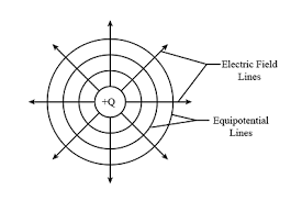
Point Charge
For a single point charge, equipotential surfaces are concentric spheres:
This means r = constant, which describes a sphere centered on the charge.
Two Equal Point Charges
For two equal point charges, equipotential surfaces have a figure-8 shape in 2D, with the midpoint being a saddle point.
Parallel Plates
For parallel charged plates, equipotential surfaces are parallel planes between the plates, with equal spacing indicating uniform electric field.
Dipole
For an electric dipole (equal and opposite charges), equipotential surfaces are more complex, with a zero-potential surface passing through the midpoint.
Visually:
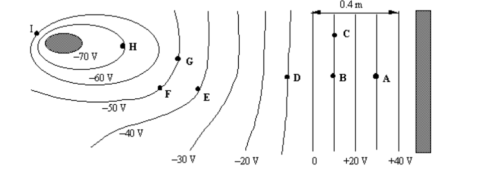
Points F and G have the same potential because they are on an equipotential line at -50 V. Also, C and B have the same potential because they are at the same equipotential line at 10 V
Relationship to Electric Field
Simple Relationship
The electric field always points from high potential to low potential, and is perpendicular to equipotential surfaces.
In simple cases (like between parallel plates or along a line):
$$E = -\frac{\Delta V}{\Delta x}$$
This means the electric field strength is the rate at which the potential changes with distance. The negative sign shows that the field points in the direction of decreasing potential.
This relationship tells us:
- Field direction: Electric field lines point from high to low potential
- Field strength: Stronger fields correspond to closer equipotential surfaces
- Uniform field: Equally spaced equipotential surfaces indicate uniform electric field
- Zero field: Widely spaced equipotential surfaces indicate weak electric field
Worked Examples
Example 1: Equipotential Surfaces for a Point Charge
Problem: A point charge of +2.0 μC creates electric potential values of 1.0 × 10⁴ V, 5.0 × 10³ V, and 2.5 × 10³ V. What are the radii of these equipotential surfaces?
Solution Steps:
- Given: q = +2.0 × 10⁻⁶ C, k = 8.99 × 10⁹ N⋅m²/C²
- Formula: \(r = k\frac{q}{V}\)
- For V = 1.0 × 10⁴ V: \(r_1 = (8.99 \times 10^9) \frac{2.0 \times 10^{-6}}{1.0 \times 10^4} = 1.8 \text{ m}\)
- For V = 5.0 × 10³ V: \(r_2 = (8.99 \times 10^9) \frac{2.0 \times 10^{-6}}{5.0 \times 10^3} = 3.6 \text{ m}\)
- For V = 2.5 × 10³ V: \(r_3 = (8.99 \times 10^9) \frac{2.0 \times 10^{-6}}{2.5 \times 10^3} = 7.2 \text{ m}\)
Answer: The equipotential surfaces are spheres with radii 1.8 m, 3.6 m, and 7.2 m respectively.
Example 2: Work Done Moving Along Equipotential Surface
Problem: A charge of +1.0 μC is moved from point A to point B along an equipotential surface where V = 5.0 × 10³ V. How much work is done?
Solution Steps:
- Given: q = +1.0 × 10⁻⁶ C, V_A = V_B = 5.0 × 10³ V
- Formula: \(W = q(V_B - V_A)\)
- Substitute: \(W = (1.0 \times 10^{-6})(5.0 \times 10^3 - 5.0 \times 10^3)\)
- Calculate: \(W = 0 \text{ J}\)
Answer: No work is done (W = 0 J) because the potential difference is zero.
Example 3: Electric Field from Equipotential Spacing
Problem: Two equipotential surfaces have potentials of 100 V and 90 V, separated by 2.0 cm. What is the magnitude of the electric field between them?
Solution Steps:
- Given: V₁ = 100 V, V₂ = 90 V, Δx = 2.0 × 10⁻² m
- Formula: \(E = -\frac{\Delta V}{\Delta x}\)
- Substitute: \(E = -\frac{90 - 100}{2.0 \times 10^{-2}}\)
- Calculate: \(E = 500 \text{ V/m}\)
Answer: The electric field magnitude is 500 V/m, pointing from the 100 V surface toward the 90 V surface.
Visualizing Equipotential Surfaces
2D Representation
In two dimensions, equipotential surfaces become equipotential lines. These are often drawn as dashed lines to distinguish them from electric field lines.
3D Representation
In three dimensions, equipotential surfaces are actual surfaces. For simple cases like point charges, these are spheres.
Computer Visualization
Modern software can create detailed 3D visualizations of equipotential surfaces for complex charge distributions.
Applications of Equipotential Surfaces
- Circuit design: Understanding equipotential surfaces helps design efficient circuit layouts
- Electrostatic shielding: Conductors form equipotential surfaces, providing shielding
- Particle accelerators: Equipotential surfaces guide charged particles
- Medical imaging: EEG and ECG measurements use equipotential surfaces
- Geophysical exploration: Mapping equipotential surfaces helps locate underground resources
Common Mistakes to Avoid
⚠️ Common Errors
- Confusing field lines and equipotential lines: Field lines are solid, equipotential lines are dashed
- Thinking equipotential surfaces can cross: They never intersect
- Forgetting the perpendicular relationship: Field lines are always perpendicular to equipotential surfaces
- Ignoring the work relationship: No work is done moving along equipotential surfaces
Practice Problems
Practice Problem 1
Problem: A point charge creates equipotential surfaces at distances of 1.0 m, 2.0 m, and 4.0 m. What are the potential values at these surfaces if the charge is +3.0 μC?
Click for solution
Solution:
- Formula: \(V = k\frac{q}{r}\)
- For r = 1.0 m: \(V_1 = (8.99 \times 10^9) \frac{3.0 \times 10^{-6}}{1.0} = 2.7 \times 10^4 \text{ V}\)
- For r = 2.0 m: \(V_2 = (8.99 \times 10^9) \frac{3.0 \times 10^{-6}}{2.0} = 1.35 \times 10^4 \text{ V}\)
- For r = 4.0 m: \(V_3 = (8.99 \times 10^9) \frac{3.0 \times 10^{-6}}{4.0} = 6.7 \times 10^3 \text{ V}\)
Answer: 2.7 × 10⁴ V, 1.35 × 10⁴ V, and 6.7 × 10³ V respectively
Practice Problem 2
Problem: Two parallel plates are separated by 5.0 cm and have a potential difference of 100 V. How many equipotential surfaces (including the plates) would you expect between them if they are equally spaced?
Click for solution
Solution:
- Electric field: \(E = \frac{100 \text{ V}}{0.05 \text{ m}} = 2000 \text{ V/m}\)
- For equal spacing: Each equipotential surface represents equal potential change
- If we want 5 surfaces: Potential difference between surfaces = 100 V ÷ 4 = 25 V
- Spacing: Distance between surfaces = 5.0 cm ÷ 4 = 1.25 cm
Answer: 5 equipotential surfaces (including the plates) with 1.25 cm spacing
Key Concepts Summary
- Equipotential surfaces are surfaces of constant electric potential
- Electric field lines are always perpendicular to equipotential surfaces
- No work is required to move a charge along an equipotential surface
- Closer surfaces indicate stronger electric fields
- Field direction is from high to low potential
- Common shapes: Spheres (point charges), planes (parallel plates), complex (multiple charges)
Quick Reference
- Work along equipotential: \(W = q\Delta V = 0\)
- Electric field from potential: \(E = -\frac{\Delta V}{\Delta x}\)
- Point charge equipotentials: \(V = k\frac{q}{r} = \text{constant}\)
- Parallel plates: Equally spaced equipotential surfaces
- Field strength: Inversely proportional to equipotential spacing